
Introduction
Recently Data Sense published an article discussing how synthetic financial data is reshaping risk management in financial services. We detailed how financial regulators have begun to experiment and publish guidelines for implementing and assessing synthetic data for analytical fidelity and privacy preservation. But how can this actually be achieved? Extending our previous research, we have provided a framework below for economists, supervisors and financial data scientists to implement and assess synthetic data use cases.
The objective of this tutorial is to help economists, supervisors, and financial data scientists gain practical experience in generating, validating, and assessing synthetic financial data using a real-world dataset, culminating in a realistic one-page briefing note.
Data and Methodology
For this tutorial we will use the World Bank World Development Indicators (WDI) dataset. We will select core macroeconomic drivers commonly referenced in supervisory work:
- GDP growth (annual %)
- Inflation, consumer prices (annual %)
- Unemployment, total (% of total labor force)
- Foreign direct investment, net inflows (% of GDP)
- Domestic credit provided by financial sector (% of GDP)
These indicators are useful for assessing fidelity because they have interpretable economic relationships. For example, Okun’s law links unemployment and output growth, allowing a straightforward check on whether synthetic data preserves the direction and relative magnitude of relationships. We will visualize these relationships and compare real vs. synthetic.
This is not private or sensitive data. That is intentional. Public data allows us to focus on analytical fidelity, and it lets us simulate privacy checks that proxy the ability to mask country-level or entity-level signals as if this were a confidential dataset.
Creating synthetic financial data. We will use the Synthetic Data Vault (SDV) library in Python. SDV provides statistical models (e.g., Gaussian Copula) and machine learning models (e.g., CTGAN). We will start with Gaussian Copula as a strong baseline for tabular data, then optionally try CTGAN for richer distributions.
Note: If no reliable real dataset is available, simulated data is an option with the SimPy library, but we will not cover simulation in this tutorial.

Part 1: Environment Setup and Data Exploration
1.1 Environment
First we need to setup our environment, if you’re using a Mac or Linux open your terminal and type the code the below. For Windows users, to activate your virtual environment use the Windows code.
python -m venv .venv
source .venv/bin/activate   # Windows: .venv\Scripts\activate
pip install pandas numpy matplotlib seaborn scikit-learn sdv wbdata1.2 Acquire and Load Data
Choose 10–15 countries and 5–7 indicators over ~20 years to keep the dataset manageable. Below is an example loader that fetches panel data from the WDI dataset.
import pandas as pd
import numpy as np
import wbdata

COUNTRIES = ['USA', 'CHN', 'JPN', 'DEU', 'IND', 'GBR', 'FRA', 'ITA', 'BRA', 'CAN', 'RUS', 'KOR', 'AUS', 'MEX', 'ESP']  # ISO 3166-1 alpha-3 codes
START, END = "2000", "2024"

INDICATORS = {
    'NY.GDP.MKTP.KD.ZG': 'gdp_growth',       # GDP growth (annual %)
    'FP.CPI.TOTL.ZG': 'inflation',        # Inflation, consumer prices (annual %)
    'SL.UEM.TOTL.ZS': 'unemployment',     # Unemployment (% of labor force)
    'BX.KLT.DINV.WD.GD.ZS': 'fdi_inflows_gdp',   # FDI net inflows (% of GDP)
    'GC.DOD.TOTL.GD.ZS': 'gov_debt_gdp'   # Central government debt, total (% of GDP)
}

# Fetch data from World Bank API
wb_data = wbdata.get_dataframe(
    indicators=INDICATORS,
    country=COUNTRIES,
    date=(START, END),
    parse_dates=True
).reset_index()1.3 Simple cleaning
Perform light cleaning and optionally apply backward/forward fill for missing datapoints or drop incomplete rows to fill out the dataset.
# Replace date with year
wb_data = wb_data.rename({"date": "year"}, axis=1)

# Ensure numeric and drop rows with all-NA features
feature_cols = list(INDICATORS.values())
for c in feature_cols:
    wb_data[c] = pd.to_numeric(wb_data[c], errors='coerce')
wb_data = wb_data.dropna(subset=feature_cols, how='all')

# Simple imputation (optional): within-country forward/back fill over time for missing datapoints
wb_data[feature_cols] = (wb_data.sort_values(['country','year']).groupby('country')[feature_cols]
                        .transform(lambda x: x.interpolate(limit_direction='both')))

# Keep complete rows for a clean baseline (skip if you imputated your data)
panel = wb_data.dropna(subset=feature_cols)
panel.head()1.4 Exploratory Data Analysis (EDA)
Describe and visualize key distributions; histograms showing the distribution of each feature, correlations of each feature, and . Focus on whether signs and rough magnitudes look plausible.
# Annova table of our panel dataset
print(panel[feature_cols].describe())
import seaborn as sns
import matplotlib.pyplot as plt
# Histograms
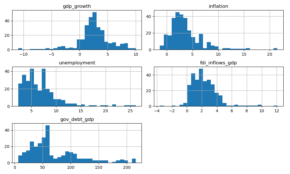
panel[feature_cols].hist(bins=30, figsize=(10,6))
plt.tight_layout()
plt.show()
# Correlations (ground truth to preserve)
corr = panel[feature_cols].corr()
plt.figure(figsize=(6,5))
sns.heatmap(corr, annot=True, cmap='vlag', center=0)
plt.title('Real Data: Correlation Matrix')
plt.show()
# Example relationship plot
plt.figure(figsize=(6,5))
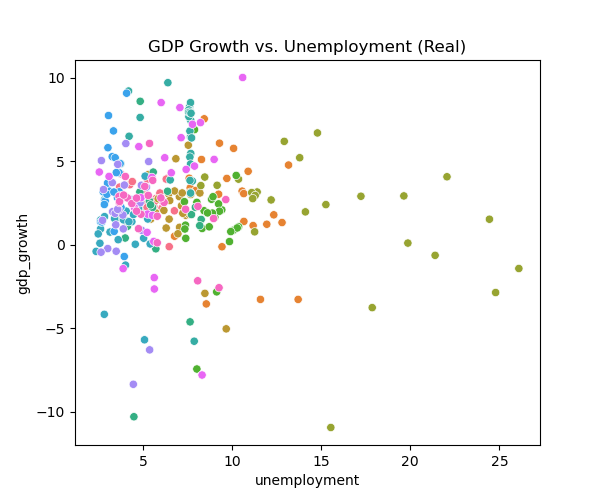
sns.scatterplot(data=panel, x='unemployment', y='gdp_growth', hue='country', legend=False)
plt.title('GDP Growth vs. Unemployment (Real)')
plt.show()
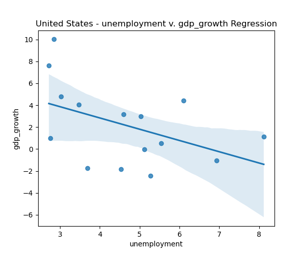
# US Okuns law example simple linear regression plot
us_data = panel.loc[panel['country'] == 'United States']
plt.figure(figsize=(6,5))
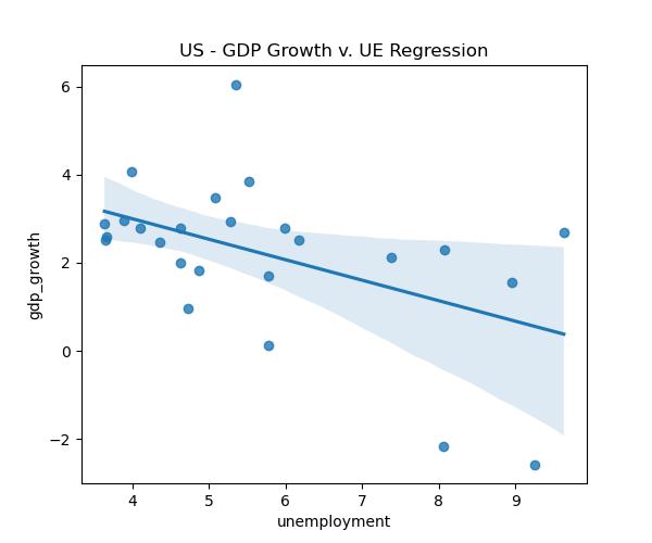
sns.regplot(data=us_data, x='unemployment', y='gdp_growth')
plt.title('US - GDP Growth v. UE Regression')
plt.show()Looking at our data, we can see that the correlation matrix shows a positive correlation between GDP growth and inflation, and negative correlation between government debt and both growth and inflation. The histograms reveal that most variables are right-skewed (except GDP growth), especially government debt, while GDP growth and inflation cluster around moderate values. The scatterplots display weak inverse relationship between GDP growth and unemployment overall, with the US regression highlighting a clearer negative slope.
ANOVA results
| Statistic | gdp_growth | inflation | unemployment | fdi_inflows_gdp | gov_debt_gdp |
|---|---|---|---|---|---|
| count | 300 | 300 | 300 | 300 | 300 |
| mean | 2.50 | 3.65 | 6.82 | 2.30 | 70.98 |
| std | 3.06 | 3.26 | 3.74 | 1.80 | 46.32 |
| min | -10.94 | -1.35 | 2.35 | -3.61 | 6.50 |
| 25% | 1.37 | 1.67 | 4.20 | 1.07 | 38.69 |
| 50% | 2.60 | 2.86 | 5.96 | 2.01 | 57.48 |
| 75% | 3.93 | 4.70 | 8.06 | 3.16 | 95.58 |
| max | 10.00 | 21.48 | 8.06 | 12.08 | 216.14 |
Graph results

Part 2: Basic Synthesis and First Validation
2.1 Define SDV Metadata
SDV benefits from explicit metadata so it handles types and constraints correctly. We can use the detect_from_dataframe function to automatically generate the necessary metadata structure.
from sdv.metadata import Metadata

metadata = Metadata().detect_from_dataframe(data=panel)2.2 Fit a Guassian Copula and Get our Synthetic Financial Dataset
First, a simple explanation of what the Guassian Copula synthesizer does:
Gussian Copula
- The Gaussian Copula synthesizer doesn’t try to copy the exact numbers; instead, it learns the dependence structure (how variables are linked) and then mixes it with the original distributions (how each variable’s values are spread out).
- This allows synthetic data generation that preserves both individual distributions and inter-variable dependencies.
In more technical terms, the Guassian Copula synthesizer models the joint distribution of our features by decoupling their marginal distributions from their dependence structure. It transforms each variable into a standard normal space using the probability integral transform, applies a multivariate Guassian distribution to capture correlations, and then maps back to the original marginals.
When fitting our Guassian Copula we have two options:
Option A (include identifiers as features):
Pass columns like country (categorical) and year (integer/time) into the model along with the numeric indicators (features). This allows SDV to learn conditional distributions (e.g., the fact that USA tends to have lower inflation than Brazil). When we generate our synthetic data, SDV can sample country + year + indicators together, preserving correlations across those identifiers.
Option B (exclude identifiers, numeric features only):
Drop country and year and fit the model on indicators only. This simplifies modeling and avoids weird synthetic years/countries (e.g. 2048), but we lose conditional structure. The synthetic data will look like “generic macroeconomic rows”. We can reattach country/year later by merging back or resampling, but the synthetic values won’t reflect per-country patterns.
Because the goal is to run real-world style analysis on the synthetic dataset, it is important to preserve relationships across countries and years. For this reason, we will use Option A and include identifiers in the synthesis. However, when experimenting with different models or running quick tests, Option B (numeric features only) can be more efficient, since it avoids the complexity of modeling categorical and temporal structure. If you decide to go with Option B, be sure to shuffle the rows in the synthetic dataset before linking back to the country and year to avoid possible linkage attacks (see 3.2 Primitive Privacy Validation).
Option A:
from sdv.single_table import GaussianCopulaSynthesizer

# Option A: include country/year
# Create synthesizer with metadata
synthesizer = GaussianCopulaSynthesizer(metadata)

# Fit on the full dataset (identifiers + features)
synthesizer.fit(panel)

# Sample synthetic data with the same shape
synthetic_data = synthesizer.sample(num_rows=len(panel))

# Sort the data by Country and Year
synthetic_data = synthetic_data.sort_values(by=['country', 'year']).reset_index()
synthetic_data.head()Option B:
from sdv.single_table import GaussianCopulaSynthesizer

# Option B (simple): fit on numeric features only
train_data = panel[feature_cols].copy()

# Get metadata for features only
metadata_feat = Metadata().detect_from_dataframe(data=train_data)

model = GaussianCopulaSynthesizer(metadata_feat)
model.fit(train_data)

# Sample synthetic data with the same shape
synthetic_data = model.sample(num_rows=len(train_data))
synthetic_data.head()2.3 Quick Visual Checks
Repeat minimal EDA to see if distributions and pairwise correlations look reasonable.
# Compare distributions
fig, axes = plt.subplots(len(feature_cols), 1, figsize=(8, 2.2*len(feature_cols)))
for i, col in enumerate(feature_cols):
    axes[i].hist(panel[col], bins=30, alpha=0.6, label='real')
    axes[i].hist(synthetic_data[col],   bins=30, alpha=0.6, label='synthetic')
    axes[i].set_title(col)
    axes[i].legend()
plt.tight_layout(); plt.show()

# Correlation comparison
fig, ax = plt.subplots(1,2, figsize=(10,4))
sns.heatmap(panel[feature_cols].corr(), annot=False, cmap='vlag', center=0, ax=ax[0]); ax[0].set_title('Real corr')
sns.heatmap(synthetic_data[feature_cols].corr(),  annot=False, cmap='vlag', center=0, ax=ax[1]); ax[1].set_title('Synthetic corr')
plt.tight_layout(); plt.show()
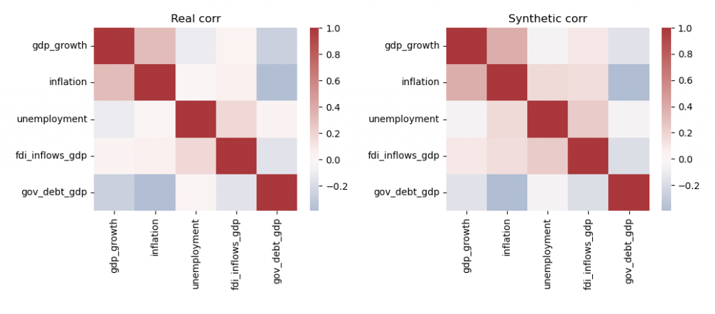
The correlation matrices show broadly similar structures between the real and synthetic datasets, though some relationships are amplified or dampened in the synthetic version. For example, the link between inflation and unemployment appears noticeably stronger in the synthetic data compared to the real data.
Histogram results
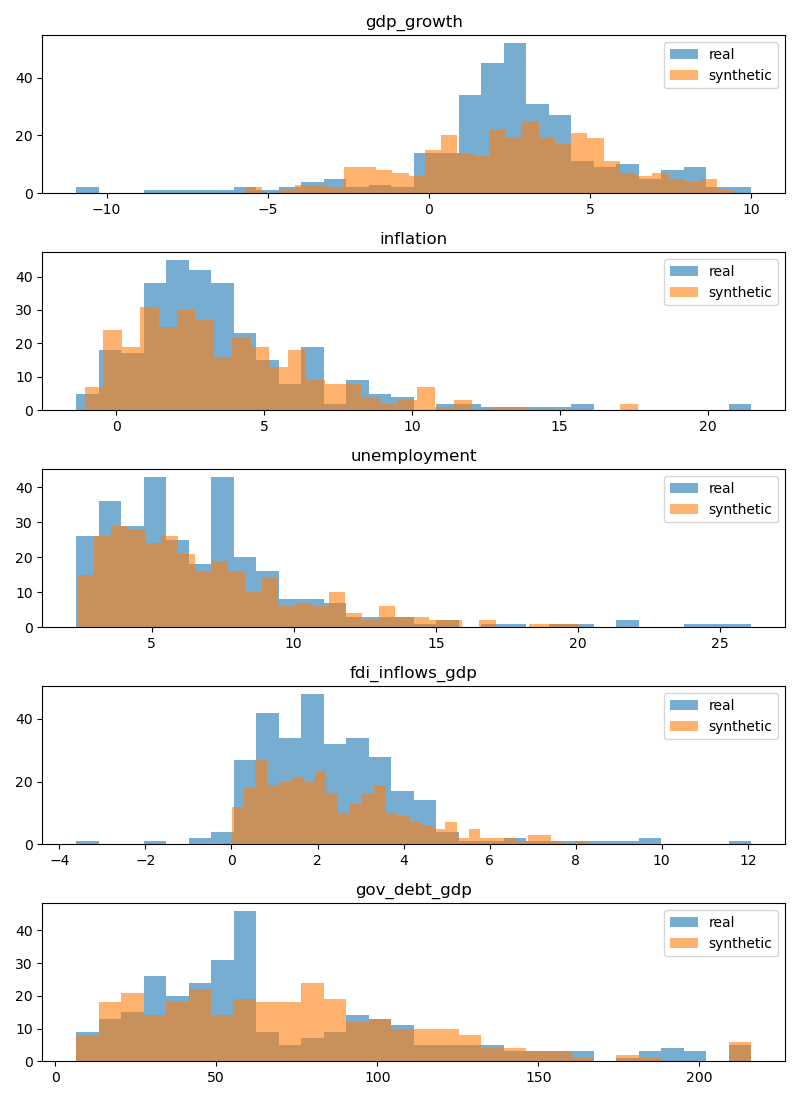
The histograms further reveal that while the synthetic dataset captures the general shape of each variable’s distribution, it tends to smooth out extremes and produce fewer outliers. This smoothing effect is expected when using a multivariate Gaussian distribution, which prioritizes capturing overall dependence structure at the expense of heavy tails and rare events. Additionally, in the second picture you can see that the relationship between US GDP and Unemployment (Okun’s law) holds in our synthetic dataset.
Takeaway
- Gaussian Copulas are useful when the goal is to preserve realistic correlations and overall distribution shapes, but they may underrepresent rare or extreme events, which is an important limitation to keep in mind for applications in finance or risk analysis.
2.4 SDV’s Built-in Quality Report (Optional)
Within the SDV library exists a diagnostic tool to assess the quality of the synthetic data versus the real dataset given the metadata, however, it’s usefulness is vague.
from sdv.evaluation.single_table import run_diagnostic

# If you used Option B replace metadata with metadata_feat
diagnostic = run_diagnostic(
    real_data=train_data,
    synthetic_data=synthetic,
    metadata=metadata
)The diagnostic returns a validity score of 100% and a data structure score of 100%… not very helpful other than to say our data is valid (no odd values) and the structure is similar to the original.
Part 3: Analytical Fidelity and Privacy Basics
3.1 Analytical Fidelity: “Same Decisions?”
We will test whether a simple linear model trained on synthetic data leads to the same directional conclusions as one trained on real data. This is aligned with the FCA’s guidelines for a “dual validation” approach, whereby above we tested the stastical significance and below we check the “fit-for-analysis”.
from sklearn.linear_model import LinearRegression
from sklearn.model_selection import train_test_split
from sklearn.metrics import r2_score
import numpy as np
import pandas as pd

TARGET = 'gdp_growth'
FEATURES = ['inflation', 'unemployment']

Xr = panel[FEATURES].values
yr = panel[TARGET].values
Xs = synthetic_data[FEATURES].values
ys = synthetic_data[TARGET].values

def fit_eval(X, y, random_state=42):
    Xtr, Xte, ytr, yte = train_test_split(X, y, test_size=0.2, random_state=random_state)
    m = LinearRegression().fit(Xtr, ytr)
    yhat = m.predict(Xte)
    return {
        'coef': m.coef_,
        'intercept': m.intercept_,
        'r2_test': r2_score(yte, yhat)
    }

real_res = fit_eval(Xr, yr)
syn_res  = fit_eval(Xs, ys)

coef_table = pd.DataFrame({
    'feature': FEATURES,
    'coef_real': real_res['coef'],
    'coef_synth': syn_res['coef'],
    'same_sign': np.sign(real_res['coef']) == np.sign(syn_res['coef']),
    'abs_diff': np.abs(real_res['coef'] - syn_res['coef'])
})
print(coef_table)
print({'r2_real': real_res['r2_test'], 'r2_synth': syn_res['r2_test']})
Results:
| Feature | Coef (Real) | Coef (Synthetic) | Same Sign | Abs. Diff |
|---|---|---|---|---|
| inflation | 0.40 | 0.34 | ✅ | 0.05 |
| unemployment | -0.06 | -0.10 | ✅ | 0.04 |
Model Fit (R²):
- Real data: -0.042
- Synthetic data: -0.027
The coefficients in the synthetic model closely track those in the real data, with the same directional effects and only small absolute differences. However, both models have negative R² values, indicating that neither provides meaningful predictive power (go figure), though the synthetic version remains directionally consistent.
We have put more a more formal test class in the Gitlab repository which outputs the results of the test along with some more structured information and assessment of the fidelity of the data.
3.2 Primitive Privacy Validation: Distance-Based Linkage Check
We will check whether synthetic records are suspiciously close to real records in normalized feature space. This is a simple proxy for assessing memorization and overfitting. To do this we will standardize the datasets and compare the rows of data using Euclidean distance.
For our sample we set a moderate threshold between 0.1 and 0.2 as the minimum distance between points. Anything under should be flagged for consideration.
from sklearn.preprocessing import StandardScaler
from sklearn.metrics.pairwise import euclidean_distances
import numpy as np

scaler = StandardScaler().fit(np.vstack([panel[feature_cols].values,
                                         synth_data[feature_cols].values]))
R = scaler.transform(panel[feature_cols].values)
S = scaler.transform(synth_data[feature_cols].values)

# Compute nearest real neighbor for each synthetic row
D = euclidean_distances(S, R)
min_d = D.min(axis=1)

summary = {
    'mean_min_distance': float(min_d.mean()),
    'median_min_distance': float(np.median(min_d)),
    'min_min_distance': float(min_d.min()),
    'pct_below_0p10': float((min_d <= 0.10).mean() * 100.0),
    'pct_below_0p20': float((min_d <= 0.20).mean() * 100.0)
}
print(summary)Results:
| Metric | Value |
|---|
| Mean Min Distance | 0.66 |
| Median Min Distance | 0.56 |
| Min Min Distance | 0.13 |
| % Below 0.10 | 0.00 |
| % Below 0.20 | 2.95 |
The average and median minimum distances (~0.66 and ~0.56) indicate that synthetic records are reasonably close to real ones in standardized space, though not identical. The minimum distance (0.13) shows that some synthetic points lie very near to real observations, but the near-zero percentages below 0.10 or 0.20 suggest that most synthetic samples are not simple replicas of real data. Overall, this implies the synthesizer preserved structural similarity without directly copying real records; a good balance for privacy and utility.
Why to worry about the results?
- > 50% below threshold: Serious memorization problem
- > 20% below threshold: Significant privacy concerns
- < 5% below threshold: Generally acceptable (some similarity expected)
We gain additional insight from the more detailed output produced by the Privacy Validation script in the Gitlab Repo. For our test case, the results are as follows:
What is a Systematic Linkage Attack?
- A linkage attack is a privacy attack where an adversary tries to “link” or match synthetic records back to real individuals in the original dataset. The attack works by:
- Assumption: The attacker has access to both the synthetic dataset and some auxiliary information about real individuals.
- Goal: Match synthetic records to real records to infer sensitive information about real people.
- Method: Use similarity measures to find the “closest” synthetic record to a known real record
Note: Our privacy preservation tests are not all-inclusive. Additional evaluations that should be incorporated include:
Membership inference attacks – current checks only assess nearest-neighbor distances, not whether an attacker could infer if a specific record was in the training set.
Attribute inference testing – no assessment of whether sensitive attributes could be inferred from non-sensitive ones in the synthetic data.
Re-identification resistance – systematic re-identification attempts were not tested, though these are increasingly considered a regulatory expectation.
Part 4: Common Failure Modes and Iteration
In order to see how our model performs when we expand our dataset, we will generate more rows of data from our real dataset and check to see if there are any obscure datapoints. This is an important consideration because Copula models do not enforce domain constraints, therefore it could generate “valid” datapoints within the distribution that are economically unintuitive such as extreme GDP growth in developed economies or negative inflation. This is a common challenge in financial applications where real-world boundaries exist.
To improve upon this, we will test a more powerful machine learning model such as CTGAN. Unlike copulas, GANs can capture complex shapes and nonlinear dependencies in the data, including distinct country-level inflation regimes. The trade-off is that GANs require more tuning, longer training times, and carry a higher risk of overfitting to real data. Another widely used model is TVAE, which we have not tested here but is a promising alternative for future comparison.
It is important to understand that generating synthetic data is an iterative process. You often start simple, identify failure modes, then refine the model or add domain constraints until the data is fit for its intended purpose. The FCA notes that domain constraints are imperative, specifically for financial data appilcations. In order to add constraints using the SDV library see the guide on implementing your own constraints.
4.1 Over-Generation and “Wonky” Values
Generate many more rows and scan for implausible values (e.g., −50% or +200% growth or inflation).
big_syn = model.sample(num_rows=len(train_data)*100)
for c in feature_cols:
    print(c, big_syn[c].min(), big_syn[c].max())
Results:
| Feature | Original Min | Synthetic Min | Original Max | Synthetic Max |
|---|---|---|---|---|
| GDP Growth | -10.94 | -9.71 | 10.00 | 10.00 |
| Inflation | -1.35 | -1.35 | 21.48 | 21.48 |
| Unemployment | 2.35 | 2.35 | 8.06 | 26.09 |
| FDI Inflows (%GDP) | -3.61 | -2.80 | 12.08 | 12.08 |
| Gov. Debt (%GDP) | 6.50 | 6.50 | 216.14 | 216.14 |
For most variables, the synthetic ranges closely align with the real dataset, capturing both lower and upper bounds. However, unemployment stands out as the Gaussian Copula model generated much higher values (up to 26%) than observed in the original data (max ~8%). This reflects how Copula methods can preserve correlations and distributional shape while occasionally producing values beyond the domain of the real data.
4.2 Trying CTGAN
CTGAN can capture more complex distributions but may require more tuning and training time.
from sdv.single_table import CTGANSynthesizer

ctgan = CTGANSynthesizer(epochs=300, metadata=metadata)  # pass cuda=True if you have an Nvdidia GPU with CUDA setup
ctgan.fit(panel)
syn_ctgan = ctgan.sample(num_rows=len(train_data))We will compare the analytical fidelity and privacy checks as per above with our CTGAN synthetic dataset this time.
Analytical Fidelity Comparison:
| Feature | Coef (Real) | Coef (Gaussian Copula) | Same Sign (GC) | Abs. Diff (GC) | Coef (CTGAN) | Same Sign (CTGAN) | Abs. Diff (CTGAN) |
|---|---|---|---|---|---|---|---|
| Inflation | 0.40 | 0.34 | ✅ True | 0.05 | -0.18 | ❌ False | 0.58 |
| Unemployment | -0.06 | -0.10 | ✅ True | 0.04 | 0.05 | ❌ False | 0.10 |
Primitive Privacy Comparison:
| Metric | Gaussian Copula | CTGAN |
|---|---|---|
| Mean Min Distance | 0.66 | 0.99 |
| Median Min Distance | 0.56 | 0.87 |
| Min Min Distance | 0.13 | 0.27 |
| % Below 0.10 | 0.00 | 0.00 |
| % Below 0.20 | 2.95 | 0.00 |
In terms of analytical fidelity, the Gaussian Copula synthetic dataset maintains the correct sign and direction of coefficients, with small absolute differences (<0.1) compared to the real data. In comparison, the CTGAN synthetic dataset struggles with fidelity, both coefficients flip sign relative to the real data, and the absolute difference for inflation is substantially larger (0.58).
On the privacy side, CTGAN produces synthetic records that are consistently farther from real ones, with higher mean and median distances and no samples within 20% of real observations. This indicates a stronger degree of privacy protection, though it comes at the cost of reduced fidelity.
Overall, the results highlight a clear trade-off: CTGAN offers stronger privacy (as reflected in the distance metrics) but weaker analytical fidelity, while Gaussian Copula delivers higher fidelity with somewhat weaker privacy guarantees, though still within our threshold of acceptability. As such, Gaussian Copula is better suited for tasks that require preservation of directional relationships and analytical structure, such as correlation analysis or supervised learning prototypes, whereas CTGAN is more appropriate when privacy takes precedence over fidelity.
These findings are consistent with the framework published by Bank Negara Malaysia for the Bank of Italy workshop in collaboration with the BIS and the IFC, which similarly ranked CTGAN and Gaussian Copula models as moderate to high on privacy preservation and low to moderate on utility. In our case, regression tests serve as a proxy for utility, reinforcing the alignment between our results and those reported in the broader regulatory literature.
Part 5: Capstone – The Regulatory Brief
Below we provide a concise one-page memo that could be handed to a manager or supervisory committee using the results and conclusions above.
Executive Summary
We generated a synthetic panel of macroeconomic indicators from the World Bank’s WDI using SDV’s Gaussian Copula, with CTGAN tested as a secondary model. In terms of analytical fidelity, the Gaussian Copula synthetic dataset preserved directional effects and produced coefficients with small absolute differences (<0.1) relative to the real data, with R² values (–0.03 vs. –0.04) close to the real-data benchmark. By contrast, the CTGAN dataset struggled with fidelity, as both coefficients flipped sign and the inflation effect showed a much larger absolute difference (0.58), alongside a weaker R² (–0.07).
Privacy screening revealed that CTGAN generated synthetic records consistently farther from real ones, with higher mean and median distances (0.99 and 0.87) and no samples within 20% of real observations. The Gaussian Copula, in comparison, produced closer matches (mean 0.66, median 0.56) with ~3% of synthetic records within the 0.20 threshold. This highlights a trade-off: Gaussian Copula offers higher fidelity but slightly weaker privacy protection, whereas CTGAN provides stronger privacy at the expense of analytical fidelity.
METHODS
Data: 15 countries, 2000–2024.
Indicators: GDP growth, inflation, unemployment, FDI inflows (% GDP), government debt (% GDP).
Models: Gaussian Copula (primary), CTGAN (comparison).
Validation: Distributional checks, correlation matrices, linear regression benchmark (target: GDP growth; features: inflation, unemployment), normalized nearest-neighbor distances for privacy screening.
Results
Utility: The Gaussian Copula preserved analytical fidelity, with synthetic vs. real correlation matrices aligned in sign and relative strength. In linear models, coefficients retained the correct sign with small absolute differences (<0.1), and R² values (real: –0.04, synthetic: –0.03) were close. By contrast, CTGAN struggled with fidelity: both coefficients flipped sign relative to the real data, with a much larger absolute difference for inflation (0.58) and a weaker R² (–0.07).
Privacy: CTGAN provided stronger privacy protection, with mean and median distances of 0.99 and 0.87 and no synthetic records within 0.20 of real observations. The Gaussian Copula, while still acceptable, generated closer matches (mean 0.66, median 0.56), with ~3% of synthetic rows within 0.20 of a real record. No exact matches were identified for either model.
Recommendations & Challenges
The Gaussian Copula is recommended for exploratory analysis, sensitivity testing, correlation studies, and training benchmarking models where directional relationships and approximate magnitudes matter more than exact values. CTGAN, by contrast, is more appropriate in settings where privacy preservation is the primary concern, such as data-sharing scenarios or prototyping with sensitive datasets. Neither model is recommended for high-stakes applications like capital allocation, policy design, or setting risk limits, since both can produce implausible extremes and, in CTGAN’s case, distort the sign and magnitude of key relationships. Looking ahead, improvements should focus on adding domain constraints to reduce unrealistic outputs, evaluating conditional synthesis by country, region, or regime, and expanding privacy testing to include membership-inference and adversarial approaches. It will also be important to compare CTGAN across multiple random seeds to assess robustness and consider hybrid methods that combine copula-based dependence modeling with GAN architectures to better balance fidelity and privacy.